Related R packages #

# spatial data analysis package
library(terra) 
# data processing package
library(tidyverse) 
# geodata encoding package
library(sf) 
# file system operation package
library(fs)

To begin with #

We need the following files for the data processing.

TIF data of nightlight intensity
Shp files are needed to identify the study area
Data description
- 4.1 shp files of administrative division in Japan, name the file jpn_adm
- 4.2 shp files link: https://data.humdata.org/dataset/cod-ab-jpn
- 4.3 nightlight tif data in Japan during 2018/09/05–2018/09/07, name the file traildata_japan, this is global data
- 4.4 data link: https://eogdata.mines.edu/nighttime_light/nightly/rade9d/

Example using trail data #

Setting and checking #

Daily nightlight tif files during 2018/09/05–2018/09/07 will be used to show how to create prefecture-level panel data using R. Before that, check the nightlight data and geo data at first.

# load tif file using 'rast' code in package 'terra'
rast("trialdata_japan/SVDNB_npp_d20180905.rade9d.tif") -> nightlight
nightlight

# load shp file
read_sf("jpn_adm/jpn_admbnda_adm1_2019.shp") -> pref
pref
vect(pref) -> pref
pref

Check files in folder ’trialdata_japan’, save the folder as ‘datafile’.

dir_ls("trialdata_japan") %>% 
  as.character() %>% 
  as_tibble() %>% 
  mutate(date = lubridate::ymd(str_match(basename(value), "\\d{8}")[,1])) %>% 
  arrange(date) -> datafile

File trialdata_japan/SVDNB_npp_d20180905.rade9d.tif, which is saved as df1, will be used an example to show the detailed steps to process nightlight tif data, while later loop will be used to operate all the nightlight files. The following R codes will also show how to use loop to deal with all the files at once on both prefecture and municipality levels

# check the name of the first file and save it as df1
datafile$value[1] 
rast(datafile$value[1] ) -> df1

Create a panel data #

Step 1: Load country, prefecture, municipality shp files

read_sf("jpn_adm/jpn_admbnda_adm0_2019.shp") %>% 
  st_transform(4326) -> jp
jp
read_sf("jpn_adm/jpn_admbnda_adm1_2019.shp") %>% 
  st_transform(4326) -> pref
pref
read_sf("jpn_adm/jpn_admbnda_adm2_2019.shp") %>% 
  st_transform(4326) -> municipal
municipal

Step 2: Use a function to calculate the statistics of the nightlight data

This is an example using one data file

# write shp data to rds data for later use
jp %>%
  write_rds("jp.rds") 
# change the data to spatial vectors
vect(jp) -> jp
# cut out the data of japan, note that this step will take time
df1 %>% 
  terra::mask(jp) %>% 
  terra::crop(jp) -> jpdf1
# check if there are extreme values using summary, such as value < 0
summary(jpdf1) 
# plot the data of japan roughly
raster::plot(jpdf1)

# calculate the mean value of nightlight by province
vect(pref) -> pref 
terra::extract(jpdf1, pref, fun = "mean", na.rm = T) -> pref_mean

# load the pref data again because spatial vectors cannot be used for merge
read_sf("jpn_adm/jpn_admbnda_adm1_2019.shp") %>% 
  st_transform(4326) -> pref
pref %>% 
  bind_cols(pref_mean) -> pref_mean
# check data (variables and data type)
pref_mean # mean value of nightlight data by prefecture in 2018/09/05

Step 3: Use loop to process all the files in folder `trialdata_japan'

In this step, package parallel is used to operate the codes by multiple lines. This loop will calculate the mean value of nightlight data on the prefecture level and municipality level.

# create new folders to save data
dir.create("pref") # create a new file named 'pref'
dir.create("municipal") # create a new file named 'municipal'

# loop to create prefecture and municipality level data
# multiple operation when data amount is large
library(parallel) 
makeCluster(3) -> cl # employ 3 operations at the same time
clusterExport(cl, "pref") 
clusterExport(cl, "municipal") 
clusterExport(cl, "jp") 
clusterExport(cl, "%>%")
clusterExport(cl, "datafile")
parLapply(cl, 1:nrow(datafile), function(x){ 
  if(!file.exists(paste0("pref/", datafile$date[x], ".rds"))) { 
    library(terra)
    # change jp data to spatial vectors
    jp <- terra::vect(sf::st_sf(jp)) 
    terra::rast(datafile$value[x]) -> nightlight 
    # cut out japan for each tif file
    nightlight %>%  
    terra::crop(jp) %>% 
    terra::mask(jp) -> nightlight
    # rule out unreasonable or extreme values
    nightlight[nightlight < 0] <- NA  
    nightlight[nightlight > 1000] <- NA 
    nightlight %>% # calculate mean values on the prefecture level
    terra::extract(terra::vect(pref), fun = mean, na.rm = T) %>% 
    tidyr::as_tibble() %>% 
    dplyr::mutate(year = x) %>% 
    # save rds file by date
    readr::write_rds(paste0("pref/", datafile$date[x], ".rds")) 
    nightlight %>% # calculate mean values on the municipality level
    terra::extract(terra::vect(municipal), fun = mean, na.rm = T) %>% 
    tidyr::as_tibble() %>% 
    dplyr::mutate(year = x) %>% 
    readr::write_rds(paste0("municipal/", datafile$date[x], ".rds")) 
    }
    }) -> nightlight_1

Step 4: Data combination after loop

# load shp files again
library(sf) 
read_sf("jpn_adm/jpn_admbnda_adm0_2019.shp") %>% 
  st_transform(4326) -> jp
read_sf("jpn_adm/jpn_admbnda_adm1_2019.shp") %>% 
  st_transform(4326) -> pref
read_sf("jpn_adm/jpn_admbnda_adm2_2019.shp") %>% 
  st_transform(4326) -> municipal

# combine nightlight data by date
library(tidyverse)
lapply(fs::dir_ls("pref"), FUN = function(x){
  readr::read_rds(x) %>%
  # delete variable 'year' 
  dplyr::select(-year)  
  }) %>% 
  bind_cols() %>% # combine by column
  # delete variables contain 'ID'
  dplyr::select(-contains("ID")) %>%  
  # add new numeric variable 'ID' 
  mutate(ID = as.numeric(row.names(.))) %>%  
  dplyr::select(ID, everything()) %>% 
  # reshape data frame
  gather(-ID, key = "key", value = "value") %>% 
  # add 'date'
  mutate(date = lubridate::ymd(str_match(basename(key), "\\d{8}")[,1])) %>% 
  dplyr::select(-key) -> prefdf # save data as 'prefdf'
# check the data
prefdf

Step 5: Write dataset to xlsx/dta file

# merge nightlight data with pref data and write to excel data
  # merge pref data to the left side of prefdf data using 'left_join'
prefdf %>% 
  left_join(
    pref %>% 
      st_drop_geometry() %>% 
      mutate(ID = as.numeric(row.names(.)))
  ) %>%  
  dplyr::select(-ID) %>% 
  # select variables to keep and reorder
  dplyr::select(date, ADM1_EN,  ADM1_JA,  ADM1_PCODE, 
                nightlight_mean = value) %>%  
  # write to excel file  
  writexl::write_xlsx("nightlight_pref.xlsx")

prefdf %>% 
  left_join(
    pref %>% 
      st_drop_geometry() %>% 
      mutate(ID = as.numeric(row.names(.)))
  ) %>% 
  dplyr::select(-ID) %>% 
  dplyr::select(date, ADM1_EN,  ADM1_JA,  ADM1_PCODE, 
                nightlight_mean = value) %>% 
  # write to dta file
  haven::write_dta("nightlight_pref.dta")

Step 6: Repeat steps 4 and 5 to output municipality level data

lapply(fs::dir_ls("municipal"), FUN = function(x){
  readr::read_rds(x) %>% 
  dplyr::select(-year)
}) %>% 
  bind_cols() %>% 
  dplyr::select(-contains("ID")) %>% 
  mutate(ID = as.numeric(row.names(.))) %>% 
  dplyr::select(ID, everything()) %>% 
  gather(-ID, key = "key", value = "value") %>% 
  mutate(date = lubridate::ymd(str_match(basename(key), "\\d{8}")[,1])) %>% 
  dplyr::select(-key) -> municipaldf 

municipaldf

municipaldf %>% 
  left_join(
    municipal %>% 
      st_drop_geometry() %>%  
      mutate(ID = as.numeric(row.names(.)))
  ) %>% 
  dplyr::select(-ID) %>% 
  dplyr::select(date, ADM1_EN,  ADM1_JA,  ADM1_PCODE,
                ADM2_EN,  ADM2_JA,  ADM2_PCODE,
                nightlight_mean = value) %>% 
  writexl::write_xlsx("nightlight_municipal.xlsx")

municipaldf %>% 
  left_join(  
    municipal %>% 
      st_drop_geometry() %>% 
      mutate(ID = as.numeric(row.names(.)))
  ) %>% 
  dplyr::select(-ID) %>% 
  dplyr::select(date, ADM1_EN,  ADM1_JA,  ADM1_PCODE, 
                ADM2_EN,  ADM2_JA,  ADM2_PCODE,
                nightlight_mean = value) %>% 
  haven::write_dta("nightlight_municipal.dta")

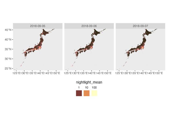
Plot to check #

nightlight distributed by municipality

library(ggplot2)
library(ggspatial)

read_sf("jpn_adm/jpn_admbnda_adm2_2019.shp") %>% 
  st_transform(4326) -> municipal
readxl::read_xlsx("nightlight_municipal.xlsx") %>% 
  mutate(date = lubridate::ymd(date)) -> mydf1 

municipal %>% 
  left_join(mydf1) %>% 
  ggplot() + 
  geom_sf(aes(fill = nightlight_mean), size = 0.001,
          linewidth = 0.001, 
          color = "white") +  
  facet_wrap(~ date, nrow = 1) + 
  scico::scale_fill_scico(
  palette = "lajolla", trans = "log10", name="nightlight") +
  scale_x_continuous(expand = c(0.001, 0.001)) +
  scale_y_continuous(expand = c(0.001, 0.001)) + 
  theme(axis.title.x = element_blank(),
        axis.title.y = element_blank(), 
        strip.text = element_text(colour = "gray30",
                                  hjust = 0.5),
        legend.position = "bottom",
        plot.margin = unit(rep(0.5, 4), "cm"),
        panel.grid.major = element_blank()) + 
  guides(fill = guide_legend(nrow = 1,
                             title.position = "top",
                             title.hjust = 0.5,
                             label.position = "top")) 
# > save as g_municipal and output jpg
# ggsave("municipalmap.jpg", g_municipal)

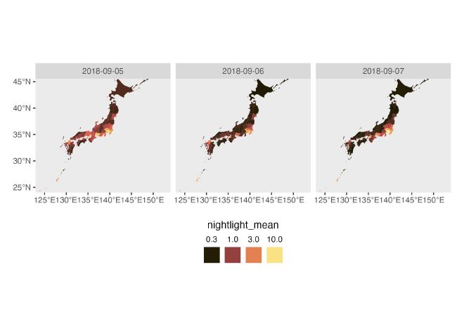
nightlight distributed by prefecture


library(ggspatial)

read_sf("jpn_adm/jpn_admbnda_adm1_2019.shp") %>% 
  st_transform(4326) -> pref
readxl::read_xlsx("nightlight_pref.xlsx") %>% 
  mutate(date = lubridate::ymd(date)) -> mydfpref1 

pref %>% 
  left_join(mydfpref1 ) %>%
  ggplot() + 
  geom_sf(aes(fill = nightlight_mean), size = 0.001,
          linewidth = 0.001, 
          color = "white") +  
  facet_wrap(~ date, nrow = 1) + 
  scico::scale_fill_scico(
  palette = "lajolla", trans = "log10", name="nightlight") +
  scale_x_continuous(expand = c(0.001, 0.001)) +
  scale_y_continuous(expand = c(0.001, 0.001)) + 
  theme(axis.title.x = element_blank(),
        axis.title.y = element_blank(), 
        strip.text = element_text(colour = "gray30",
                                  hjust = 0.5),
        legend.position = "bottom",
        plot.margin = unit(rep(0.5, 4), "cm"),
        panel.grid.major = element_blank()) + 
  guides(fill = guide_legend(nrow = 1,
                             title.position = "top",
                             title.hjust = 0.5,
                             label.position = "top")) 
# > save as g_pref and output jpg
# ggsave("prefmap.jpg", g_pref)

Causal Forest

Stata R Causal Forest